Confusion Matrix Function in R Continuous Variable

A confusion matrix in R is a table that will categorize the predictions against the actual values. It includes two dimensions, among them one will indicate the predicted values and another one will represent the actual values.

Each row in the confusion matrix will represent the predicted values and columns will be responsible for actual values. This can also be vice-versa. Even though the matrixes are easy, the terminology behind them seems complex. There is always a chance to get confused about the classes. Hence the term -Confusion matrix

In most of the recourses, you could have seen the 2x2 matrix in R. But note that you can create a matrix of any number of class values. You can see the confusion matrix of two class and three class binary models below.

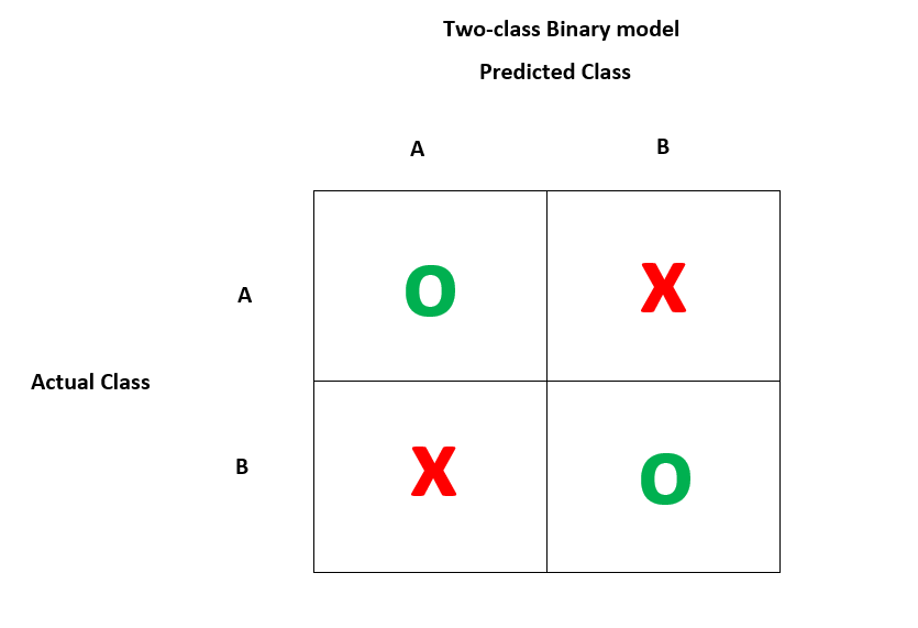
This is a two-class binary model shows the distribution of predicted and actual values.

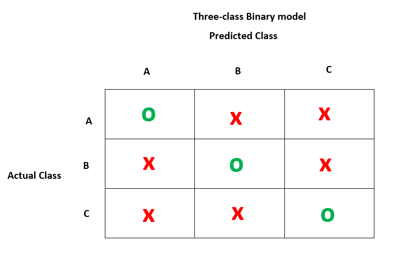
This is a three-class binary model that shows the distribution of predicted and actual values of the data.

In the confusion matrix in R, the class of interest or our target class will bea positive class and the rest will benegative.

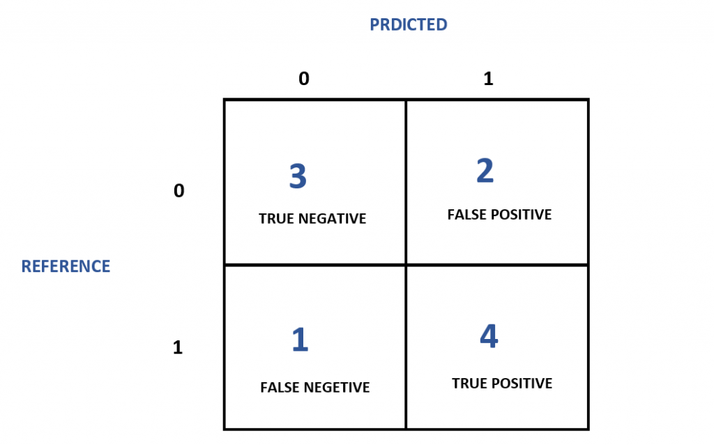
You can express the relationship between the positive and negative classes with the help of the 2x2 confusion matrix. It will include 4 categories -

• True Positive (TN) - This is correctly classified as the class if interest / target.
• True Negative (TN) - This is correctly classified as not a class of interest / target.
• False Positive (FP) - This is wrongly classified as the class of interest / target.
• False Negative (FN) - This is wrongly classified as not a class of interest / target.

Creating a Simple Confusion matrix using R

In this section, we will use the demo number data which we are going to create here. Here, our interest/target class will be 0.

Let's see how we can compute this using the confusion matrix. You can set the target class as 0 and observe the results.

It will be a bit confusing, but take your time and dig deep to get it better. Let's do this using the caret library.

                      #Insatll required packages            install.packages(            'caret'            )            #Import required library            library(caret)            #Creates vectors having data points            expected_value            <-            factor(c(            1            ,            0            ,            1            ,            0            ,            1            ,            1            ,            1            ,            0            ,            0            ,            1            )            )            predicted_value            <-            factor(c(            1            ,            0            ,            0            ,            1            ,            1            ,            1            ,            0            ,            0            ,            0            ,            1            )            )            #Creating confusion matrix            example            <-            confusionMatrix(data=predicted_value,            reference            =            expected_value)            #Display results                        example                  

          Confusion Matrix and Statistics                 Reference Prediction      0    1             0   3    2             1   1    4                                                           Accuracy : 0.7                               95% CI : (0.3475, 0.9333)     No Information Rate : 0.6                  P-Value [Acc > NIR] : 0.3823                                                                        Kappa : 0.4                                                          Mcnemar's Test P-Value : 1.0000                                                                  Sensitivity : 0.7500                       Specificity : 0.6667                    Pos Pred Value : 0.6000                    Neg Pred Value : 0.8000                        Prevalence : 0.4000                    Detection Rate : 0.3000              Detection Prevalence : 0.5000                 Balanced Accuracy : 0.7083                                                             'Positive' Class : 0                  

Woo!!! That's cool. Now I am sure that things are pretty much clear at your end. This output alone can answer tons of questions that are rolling in your mind right now!

Measuring the performance

The success rate or the accuracy of the model can be easily calculated using the 2x2 confusion matrix. The formula for calculating accuracy is -

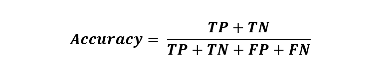
Here, the TP, TN, FP, AND FN will represent the particular value counts that belong to them. The accuracy will be calculated by summing and dividing the values as per the formulae.

After this, you are encouraged to find the error rate that our model has predicted wrongly. The formula for error rate is:

The error rate calculation is simple and to the point. If a model will perform at 90% accuracy then the error rate will be 10%. As simple as that.

The simple way to get the confusion matrix in R is by using the table() function. Let's see how it works.

          table(expected_value,predicted_value)                  

                      predicted_value expected_value         0        1                  0     3        1                  1     2        4                  

Let me make it much more beautiful for you.

Perfect! Now you can observe the following points -

• The model has predicted 0 as 0, 3 times and 0 as 1, 1 time.
• The model has predicted 1 as 0, 2 times and 1 as 1, 4 times.
• The accuracy of the model is 70%.

Confusion matrix using "gmodels"

If you want to get more insights into the confusion matrix, you can use the 'gmodel' package in R.

Let's install the package and see how it works. The gmodels package offer a customizable solution for the models.

                      #install required packages            install.packages(            'gmodels'            )            #import required library                        library(gmodels)            #Computes the crosstable calculations            CrossTable(expected_value,predicted_value)                  

                      Cell Contents |-------------------------| |                       N | | Chi-square contribution | |           N / Row Total | |           N / Col Total | |         N / Table Total | |-------------------------|    Total Observations in Table:  10                    | predicted_value  expected_value |         0 |         1 | Row Total |  ---------------|-----------|-----------|-----------|              0 |         3 |         1 |         4 |                 |     0.500 |     0.500 |           |                 |     0.750 |     0.250 |     0.400 |                 |     0.600 |     0.200 |           |                 |     0.300 |     0.100 |           |  ---------------|-----------|-----------|-----------|              1 |         2 |         4 |         6 |                 |     0.333 |     0.333 |           |                 |     0.333 |     0.667 |     0.600 |                 |     0.400 |     0.800 |           |                 |     0.200 |     0.400 |           |  ---------------|-----------|-----------|-----------|   Column Total |         5 |         5 |        10 |                 |     0.500 |     0.500 |           |  ---------------|-----------|-----------|-----------|                  

That's amazing! You can see plenty of information that the gmodel library has returned based on the given data. It's plenty of information right?

Time for calculation using confusion matrix

Finally, it's time for some serious calculations using our confusion matrix. We have defined the formulas for achieving the accuracy and error rate.

Go for it!

          Accuracy = (3 + 4) / (3+2+1+4)                  

          0.7 = 70 %                  

The accuracy score reads as 70% for the given data and observations. Now, it's straightforward that the error rate will be 30%, got it?

If not, we can go through our formula.

          Error rate = (2+1) / (3+2+1+4)                  

          0.30 = 30%                  

Cool! The model has wrongly predicted 30% of the values. The error rate is 30%.

This is also equal to the formula -

          error rate = 1 - accuracy                  

          1 - 0.70 = 0.30 = 30%                  

You can simple minus the accuracy value with 1 to get the error rate. Things are going pretty much easy though!

Wrapping Up

A confusion matrix is a table of values that represent the predicted and actual values of the data points. You can make use of the most useful R libraries such as caret, gmodels, and functions such as a table() and crosstable() to get more insights into your data.

A confusion matrix in R will be the key aspect of classification data problems. Try to apply all these above-illustrated techniques to your preferred dataset and observe the results.

That's all for now. Happy R!!!

More read: R documentation

winegarfick1992.blogspot.com

Source: https://www.digitalocean.com/community/tutorials/confusion-matrix-in-r

Share this post